A finite difference equations allows to obtain the new value for a given variable, from the current value, as a function of discrete time steps. This functional relationship can be written as $$ x_{t+1}=f(x_t) $$ where the function $f$ characterizes the mapping. sometimes, $x_{t+1}$ is denoted as $x'$.
For example, let's assume a linear equation, $x_{t+1}=Rx_{t}$, where $R$ is a constant. What is the solution of this equation?
In this case the solution is easily obtained, and for a given initial condition $x_0$, you have $$x_1=Rx_0,$$ $$x_2=Rx_1=R^2 x_0,$$ $$x_{t}=Rx_{t-1}=R^2 x_{t-2} = \ldots =R^t x_0$$. therefore, the solutions behaviour is completely encoded in the parameter $R$. You will see that a very rich dynamics can be spanned by the given parameters. You have the following possible solutions, as function of time:
import matplotlib.pyplot as plt
import numpy as np
N = 40
def iterate(data, R):
    for i in range(1, N):
        data[i] = R*data[i-1]
# Iteration settings
t = np.arange(0, N)
xdata = np.zeros(N)
xdata[0] = 0.5
# plot settings
fig, ax = plt.subplots(figsize=(8,6))
# Maps for several values of R
R = -1.01
iterate(xdata, R)
plt.plot(t, xdata, label=r'$R < -1$')
R = -0.8
iterate(xdata, R)
plt.plot(t, xdata, label=r'$-1 < R < 0$')
R = +0.8
iterate(xdata, R)
plt.plot(t, xdata, label=r'$0 < R < 1$')
R = +1.0
iterate(xdata, R)
plt.plot(t, xdata, label=r'$1 = R $')
R = +1.01
iterate(xdata, R)
plt.plot(t, xdata, label=r'$1 < R $')
plt.legend()
plt.show()
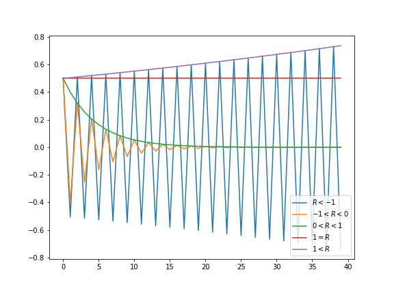
After checking the solution and looking at this behaviour, you can easily conclude that:
- For $|R|>1$, the state variable grows in time, unbounded. For negative values, you also have oscillations (of increasing amplitude). this is valid for any initial condition $x_0\neq 0$.
- For $|R|<1$ the system decays to zero in spite of the initial condition. Therefore, the point $x=0$ is a limit point and stable, for this values of $R$. Any initial condition will end at that point, after enough iterations.
- Remaining cases are, for example, steady when $R=1$. In this case any point is a fixed point, since $x_{t+1}=x_t$ for all iterations.
The stability (sensitivity to small perturbations) of points can be explored analytically by the behaviour of the first order derivatives (linearization). Furthermore, what will be important is the stability of the fixed points, that is , the points which fulfill xt+1=xt (which is the same as dx/dt=0 for a continous map), something which can be obtained after a few or after many iterations.
the Logistic map
The logistic map has been used to model several kind of systems and its origins are related to the study of the population dynamics. Imagine that $x_t$ denotes the population of certain system at time $t$. One expects that if the population is small, then it will grows proportionally to the current population, $x_{t+1}\propto x_t$. But, if the population is too large, then competition for resources will decrease the population, $x_{t+1}\propto 1−x_t$. Therefore, one can model the population as
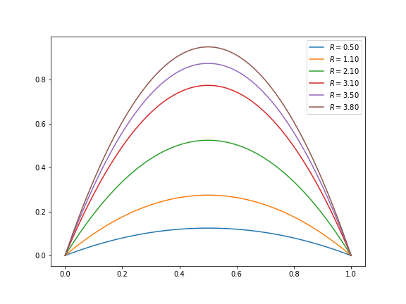
$$ x_{t+1} = Rx_t (1-x_t)$$This is the logistic maps, and its simplicity hides a very rich behaviour. A typical figure (for a normalized) is as follows
#include <iostream>
#include <vector>
#include <cstdlib>

// call: ./a.out NITER R
int main(int argc, char **argv)
{
  const int NITER = std::atoi(argv[1]);
  const double R = std::atof(argv[2]);
  std::vector<double> x(NITER);

  x[0] = 0.12;
  for (int ii = 1; ii < NITER; ++ii) {
    x[ii] = R*x[ii-1]*(1-x[ii-1]);
  }

  for (int ii = NITER/2; ii < NITER; ++ii) {
    std::cout << ii << "  " << x[ii] << "\n";
  }

  return 0;
}
To run the cpp code for several values of R, you use a bash loop,
for R in 0.5 1.1 2.1 3.1 3.5 3.8; do echo "R = $R"; ./a.out 100 $R > datos-$R.txt ; done
Then we plot with python
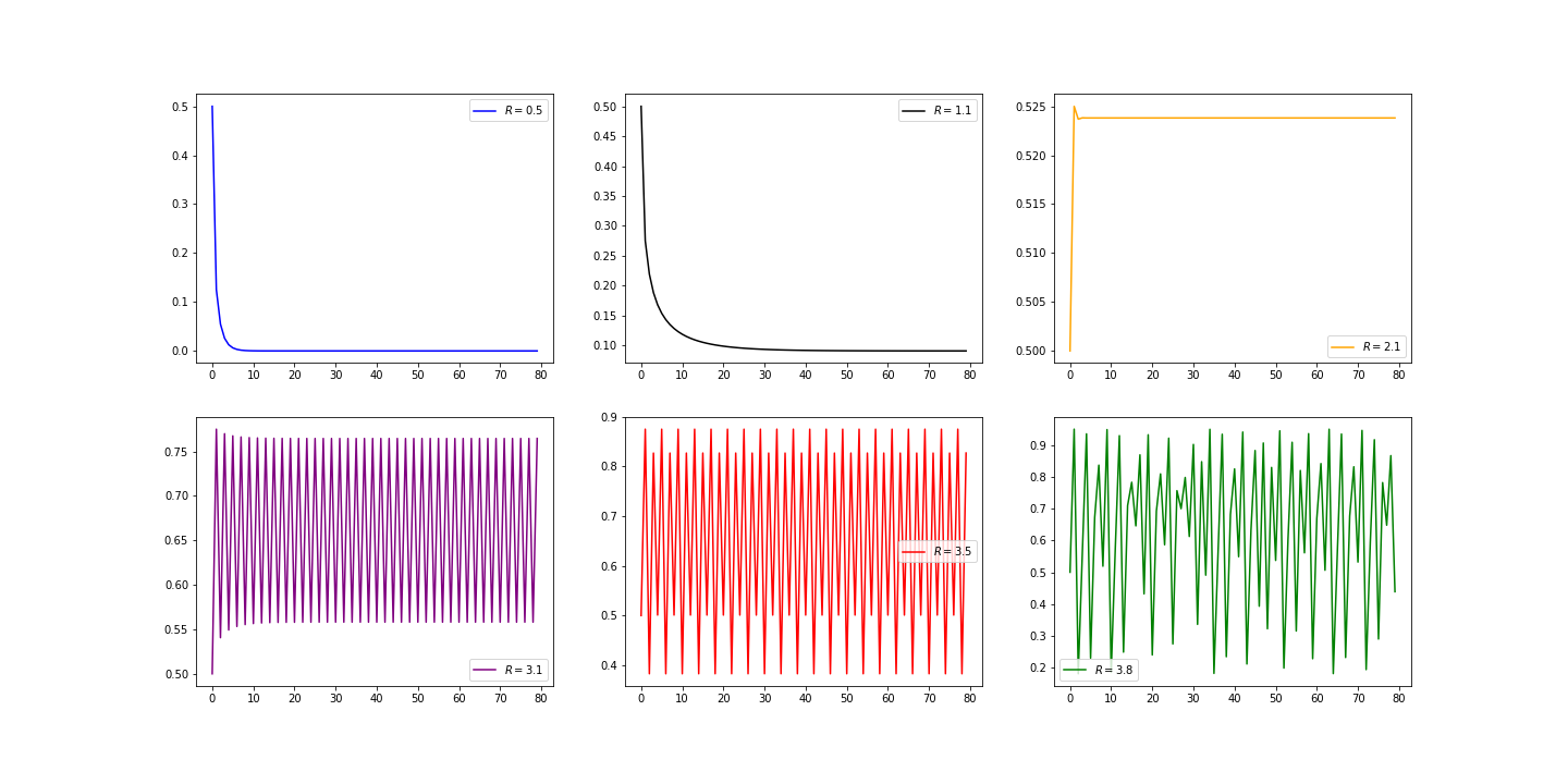
As you can see, the actual behaviour of the solutions is very different from the linear map, and there are some ranges for R where the solutions is steady, decaying, periodic, and non-periodic.
As you can see, the actual behaviour of the solutions is very different from the linear map, and there are some ranges for R where the solutions is steady, decaying, periodic, and non-periodic.
Actually, it is uncommon to focus on the $x_t$ vs. $t$ plot, since it can hide a lot of information. For example, how can you now that actually you are looking at some steady state? or you need to perform more iterations? In these cases is customary to rely on return maps or phase portraits, that is, plots of $x_{t+1}$ vs. $x_t$. In this case is easy to check if the system is reaching a single point, like $x=0$, or a periodic orbit, or something much strange (like a fractal). Let's plot the return map for the previous values of $R$.
But we could see the behaviour of this at every step, we could see that for some values of $R$ we have "sinks", for example let's run in python our own program for value of $R=2$
def Logistic_map(x,L):
    return L*x*(1-x)
x=[0.001]
R=2
for i in range(100):
    x.append(Logistic_map(x[-1],R))
    plt.step(x,x,alpha=1,color="rebeccapurple",linewidth=0.8)
    plt.title(r"$\lambda=${}, iteration number = {}".format(round(R,3),i+1)))
    plt.plot(x_total,Logistic_map(x_total,R),color="navy")
    plt.plot(x_total,x_total,color="orange")
    plt.xlim(0,0.6)
    plt.ylim(0,0.6)
    plt.show()

Or for different values of $R$ we have
17.3 Local stability and fixed points
A fixed point is a point where $x_{t+1}=f(x_t)=x_t$ (or, for continuous equations, $0=dx/dt$). The behavior of small perturbations around this points are related to the stability of the fixed point. If the small perturbations separates from the point, the point is said to unstable. Otherwise it is stable.
Let's assume the existence of a fixed point, $x_p$. A small perturbation around it can be written as $\eta=x_t−x_p$, therefore, $\eta_{t+1}=x_t+1−x_p=f(x_t)−x_p=f(\eta+x_p)−x_p=f(x_p)+f′(x_p)\eta_t−x_p=f′(x_p)\eta_t$. In other words, $\eta_{t+1}/\eta_t=f′(x_p)$. Therefore, if $|f′(x_p)|>1$, the point is unstable; else, if $|f′(x_p)|<1$, the point is stable (The equivalent for continuous functions is with $f′(x_p)>0$ etc).
Exercise
Compute the fixed points and the stability for Logistic map
If a point is locally stable, then some iterations would be needed to reach it. Those iterations are called the transient.
The set of local initial conditions which reach the same limit fixed point is called the basin of attraction of the fixed point. They can have a very complicated geometry.
Cycles
A cycle or $n$ -order is a trajectory which repeats itself, defined as
$$x_{t+n}=x_t$$but $x_{t+j}\neq x_t$, for $j=1,2,3,…,n−1.$
A fixed point is a cycle of period 1. A cycle of period 2 is defined as $x_{t+2}=f(x_t)=f(f(x_t))$. If the function $x_{t+1}=f(x_t)$ has a period-2 cycle, then the function $f(f(x_t))$ has, at least, two fixed points. Longer cycles can be found similarly: "just" solve the equation
$$x_t=\underbrace{f(f(\cdots f(x_t)\cdots))}_{\text{n times}}$$Introduction to chaos
A deterministic system can present chaotic behaviour, showing the following characteristics:
- Aperiodicity.
- Bounded solutions.
- Deterministic.
- Sensitive dependence on initial conditions.
An example of this can be found using two different initial conditions and a $R=4$
In order to determine when the system becomes chaotic we can do something called a bifurcation diagram. To do this we are based in the fact of existence of fixed points, meaning that if we reach the transient limit for many conditions we should have that the result have to end up in a fixed point.
- We use many initial conditions from 0 to 1 (Why?)
- Let evolve all those conditions enough to reach its transient value.
- Plot the final value after applying the map several times.
this can be easily done in python using the following code:
plt.figure(figsize=(20,20))
for L in np.linspace(1,4,1000):
    x=np.linspace(0.0001,1,10000)
    for i in range(1000):
        x=Logistic_map(x,L)
    plt.plot([L]*len(x),x,".",markersize=0.01,color="k")
    plt.ylim(0,1)
    plt.xlim(1.5,4)
plt.show()
for more resolution check this link
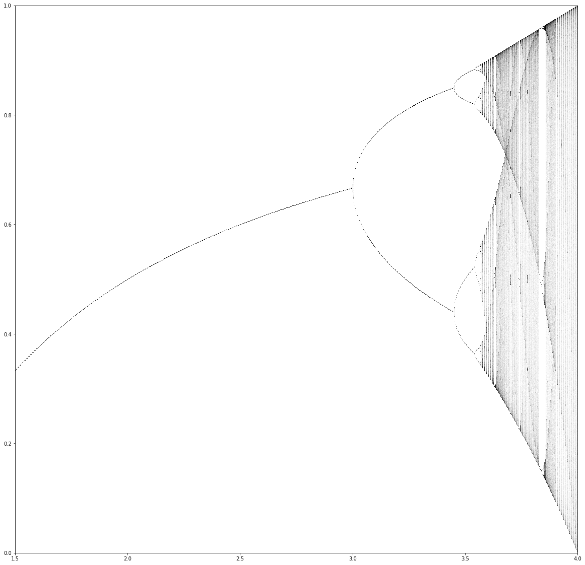
There are several observations we can extract from this examples:
- The system is chaotic only for some values of the parameter R (which ones?).
- You can see (R=3.0) the existence of some transient time before the system settles to a periodic behaviour.
- There are some period doubling results when changing the parameter R (check R=3.0 and R=3.5).
- Close values of R do not necessarily produce the same behaviour (check R=3.800 and R=3.801).
Regarding the period doubling, it has actually been found that the logistic map shows what is called a period-doubling route to chaos. Actually, there are successive period-doublings as $R$ changes, with values $2$, $4$, $8$, $16$, $32$, and so on. If $R_n$ denotes the value at which a $2n$ -cycle appears, the numerics reveals that (see Strogatz et. al.) $R_1=3$ generates a period 2-cycle, $R_2=3.449…$ a 4-cycle, $R_3=3.54409…$ a period-8, $R_4=3.5544…$ a period-16, $R_5=3.568759…$ a period-32, …, and $R_{\infty}=3.569946…$ a period-$\infty$ cycle.
Successive period-doublings come faster, and it can be shown that the convergence is geometric, and the convergence rate can be characterized by a single constant,
$$ \delta =\lim_{n\to\infty}\frac{R_{n}-R_{n-1}}{R_{n+1}-R_{n}} = 4.669\ldots $$This is called the Feingenbaum constant, and seems to be a universal constant which characterizes the route to chaos in many systems.
Exercise (Optional)
Do all we have done until now for the next two maps (Everything in c++ and use python only to plot):
Tent map $$x_{t+1}=R \min\left( x_{t},1-x_{t}\right)$$
Sine map $$ x_{n+1} = R \sin(\pi x), \quad x\in [0,1], \mu >0.$$